Creating Distance Buffers

Vector data model

Distance buffers around lines or polygons are not simply parallel lines or parallel polygons around the object at a certain distance. To create buffers additional circular arcs with radius l are required. The following animation shows the construction of a distance buffer a line.

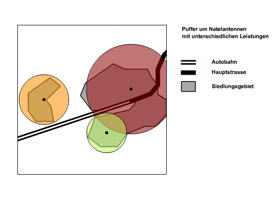
Distance buffers around points are circles. The points presented in the following illustration, represent the location of mobile phone antennas with different transmission power. Thereby, the furthermost line is the maximal range at a given transmission power. The distance buffers are weighted with attribute values of the object. On the map, the regions of the settlement area that are within the transmission range and which are outside of the transmission range, are indicated.

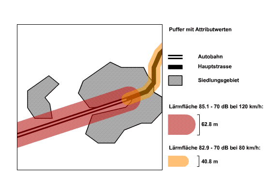
The next two examples deal with distance buffers around lines. In these two cases, the lines represent roads of different classes. Due to the classification of the roads, the speed limits are known: Highway 120km/h and main road 80km/h. According to an immission / emission model for street noise (cf. Laermorama), the distance buffers were calculated for a limit value of 70dB depending on the speed limit. There are mainly three parameters integrated in the model: Average speed, average number of vehicles per hour and the percentage of trucks. Obstacles were not considered. It is assumed that the sound propagates unimpeded in space. The resulting area covers the region of 85.1dB at the major artery and 70dB at the outline of the distance buffer (respectively 82.9dB to 70dB). This means that the buffered area is not homogeneous with respect to the immission value. Often, the boundary respectively the limits are of interest. The resulting buffered area is useful to answer to questions such as: How big are the affected areas and how many inhabitants are influenced by the noise?

If you want to represent the immission values gradually, various distance buffers with the respective immission values have to be calculated. To avoid, that the areas always start at 85.1dB, the buffer polygons have to be overlaid. You can learn more about polygon overlay in the lesson "Suitability Analysis".

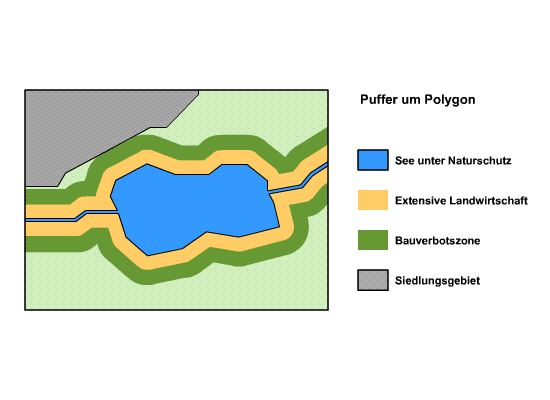
The last example shows one-sided distance buffers. They have been determined based on a law. They define the area around the nature reserve, where only extensive agriculture is allowed and where a construction ban is established.

Raster data set

Have a look at the following animation. In the first illustration, the cells of the tram stop are indicated with the value 7. Starting at these two "source cells", for each cell in the grid the distance to the nearest "source cell" is calculated. The result of this calculation is a "distance raster". In this resulting raster, the distance assigned to the "source cells" is 0. The transformation is based on the Euclidean distance. In the animation, the values can be reclassified. Thus, a quasi continuous surface, containing noise values, could be generated. The accuracy and the continuity of the raster depend on the raster resolution. Noise zones could be established by reclassifying the immission values.

Greater

In a raster data model, distance transformation can be performed for areas or any arrangement of "source cells". In the example below, the grid cells are of the same thematic, coded with the value 99, representing a forest. For each cell, the shortest path to the edge of the forest can be calculated (depending on the metric). The results are entered in a new raster. In this new raster, the values assigned to the cells represent the distance to the edge of the forest. At the edge of the forest, the values are smaller and increase to the center. In our example, the Manhattan metric was chosen. Consequently, only the direct neighbors of a cell (4 neighbors) are included to the calculation. Thus, the region is transformed stepwise, one cell width after the other. The results of each calculation step are joined and added to a common raster. You can learn more about the combination of raster in the lesson "Suitability Analysis".

Greater