Primitives of a Network

Terms of graph theory and networks

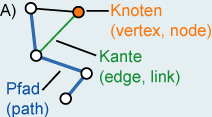
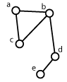
In graph theory, distinct terminology may apply. However, most terms have simple definitions. A graph consists of two types of elements, namely vertices (V) and edges (E) (e.g.: Graph A). Vertices represent objects that can have names and other attributes such as, for example, transfer points in a subway system. Every edge has two endpoints in the set of vertices, and is said to connect or join the two endpoints (they are adjacent), e.g. a flight connection between Zurich and Berlin. 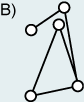Graphs are represented by drawing a dot or circle for every vertex, and drawing an arc between two vertices if they are connected by an edge (Graphs A-K). A graph is defined independently from its visualisation. Both figures A and B display the same graph.
A path from vertex s to vertex e in a graph is a list of adjacent vertices. A simple path is a path where no vertex is used more than once. In a connected graph there is an edge from each vertex to every other vertex. In a disconnected graph, there are disconnected parts of edges and nodes (Graph C).

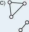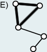
Elements of a graph	Connected graph	Disconnected graph

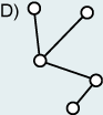
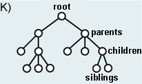
A cycle is a simple path where the first and last vertex is the same (Graph E). A graph without cycles is called a tree (Graph K). Trees have a hierarchical structure and are often explicitly displayed.
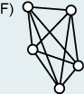
The complete graph is a simple graph in which each vertex is adjacent to every other vertex (Graph F).
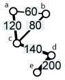
Graphs are considered as sparse when they have a relatively small number of edges; graphs with a small number of possible edges missing are described as dense. In weighted graphs (Graph G), a number or a weight is assigned to each edge of the graph to represent distance (temporal or geometric) or cost. That way, more information is linked to the graph.

Undirected Graphs:

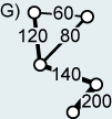	Cycle	Complete graph	Weighted graph

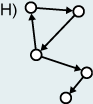
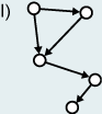
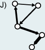
In directed graphs, edges are "one-way streets" (Graph H); an edge can lead from x to y but not from y to x. Directed graphs without directed cycles (directed cycles: all edges point in the same direction) are called directed acyclic graphs (Graph I). Directed and weighted graphs are called networks (Graph J). In colloquial language and in the field of geography the term net or network is often used for all kinds of graphs.

Directed Graphs:

Graph with a cycle	Acyclic	Directed and weighted = Network	Hierarchic

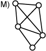
There is another categorization: planar and non-planar graphs. A planar graph is one which can be drawn on the plane without any lines crossing (Graphs L and M).

Planar vs. non-planar graphs:

Planar	Non-planar

Another simple form of representation for graphs, which can also be processed by a digital computer, is an adjacency matrix. A matrix of size VxV is designed, where V is the number of nodes. The fields are set to 1 if an edge between the nodes exists, for example, a and b, and to 0 if no such edge exists. In the example we assume that an edge from each node to itself exists. Whether you set the size of the diagonal to 1 or 0, depends on the intended purpose. In some cases it is better to set the diagonal to 0. This matrix is called adjacency matrix because its structure indicates which nodes are neighbouring (i.e. are adjacent). Something similar is possible with weights: the weights (instead of the value 1) are written into the fields.

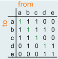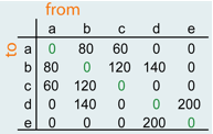Adjacency matrix	Matrix with weights

The notion of topology is often used in associtation with the description and analysis of networks. Topology and its concepts are discussed in detail in the module "Spatial Modeling". The networks shown in the figure below have topologically equivalent compounds, thus they are topologically equivalent graphs.

Two topologically equivalent graphs