Illustration with the movement of a walker

For didactical purposes this section is organised as follows: Principles of accessibility modelling are presented in turn for the three levels of modelling space and its properties. A common example will illustrate for these three levels the movement of a walker. This specific situation is characterised by an active moving person with an internal force, by a moving strategy that is influenced by several factors related with individual properties of places in space.

This rather simple example should be familiar to most of us and is suitable for the three levels of models. Let us describe the situation of this illustration. A person wishes to walk from a starting place –an origin- to a destination within our imaginary region of Examplis. Its topography is moderate with a heterogeneous landcover. Next figure illustrates the topography and the landcover of this region and shows the origin (O) and the destination (D) of the walker’s movement.

Modeling movement in an isotropic plane surface

In this modeling context, only geometric properties are influencing the movement of the walker. The measure of distance between locations in space, their proximity and the length of the path are expressed with metric units.
Principal characteristics of the model at this level are the following:

• The distance to the destination increases linearly and homogeneously in all directions as a function of the proximity to this location. These two characteristics of regularity and isotropy correspond graphically to a concentric distribution of distances with maximal values on the corners of the region (figure 3.26a).
• According to the Euclidian geometry rules, the optimal path between the origin and destination is a line linking them.

We can observe on next figure a) that space is considered as homogeneous in this model and therefore only the geometric distance is considered for the estimation of proximity from any place to the destination. This is confirmed with the overlay of the optimal path onto the landcover distribution (figure b). One can observe that there is no influence.

Modeling movement in an isotropic skewed surface

For this modeling context, it is possible to take into account both the Euclidian distance from the geometric dimension and the friction effect due to individual properties of space in the thematic dimension. It is then necessary to construct a layer of friction coefficients that express the friction effect of each cell on the movement of the walker.

In this application let us limit the consideration of a single friction factor to the movement: the cover at the surface of the land. Our concern is to translate the landcover properties in terms of friction effect. Let us choose a cost distance unit as the time unit in minutes and therefore call this distance a time distance. The coefficient friction value attached to each cell corresponds to the amount of time necessary to cross this cell according to its landcover friction effect. Assuming a cell size of 100m, the friction value assigned to each landcover type is listed in the next figure. The production of the friction layer illustrated in the next figure is based on a simple classification of landcover types into minutes. We can observe that the road cover has the lowest friction coefficient, the marshy cover a high value and water covers have an infinite friction value, corresponding to an impermeable barrier.

The computation of the time distance from each cell to the destination cell can now be started through an iterative and cumulative process from the destination to all image cells. The GIS software Idrisi offers such a procedure called COST-GROW. The next figure a) shows the optimal path of the walker overlayed onto the time distance image. One can observe that the most distant location is no more than four image corners, like with the Euclidian distance, but the southern part of the river that flows through the marshy cover . In figure b) the optimal path has been overlaid onto the landcover image in order to illustrate the influence of the considered friction factor on the optimal path.

Modeling movement in an anisotropic skewed surface

In the third level of this model of space, the heterogeneity of friction properties can be taken into account. Let us consider the factor topography to illustrate the anisotropic friction effect. By experience we should admit that the slope of a cell has not the same influence when walking downhill or uphill. The slope steepness of that cell is identical, but its friction effect varies according to the direction of movement of the walker relatively to the direction of the slope. If we consider more carefully the effect of this topography factor we can observe that in direction of the steepest descending slope the friction effect is in fact transformed into a force –the gravity force- that aids to walker to move across the cell. In other words, this anisotropic characteristic allows us to consider friction factors for which friction varies as a function of the direction of movement. As you remember we have admitted that the influence of a factor acting either as a force or a friction can be modeled with a unique concept of relative friction. In order to model this influence we can consider a force-friction vector made of two components: its intensity and a function of directional variability.

Let us return to our application of modeling the movement of our walker. Our objective is to consider the effect of both the landcover and the topography along with the walking time and pathway. Let us proceed in two steps, first we concentrate on the modeling of the topographic factor and in the second step we combine its joint influence with the landcover factor previously discussed.

The factor topography with anisotropic properties The force-friction effect on the walker’s movement is a function of the direction of walking with respect to the direction of the slope on each piece of terrain: a cell. The next figure illustrates the strength of this effect for different relative directions noted Δα. We can then identify three typical situations:

• Up hill situation: When the direction of movement matches the direction of the steepest slope, the relative angle Δα = 0° and therefore the friction effect of the slope is maximal.
• No slope situation: When the direction of movement is perpendicular to the direction of the steepest slope, the relative angle Δα = 90° or 270° and the slope effect is neutralized. Therefore the friction effect of the slope is unitary (=1), corresponding to a flat surface.
• Downhill situation: When the direction of movement is opposite to the direction of the steepest slope, the relative angle Δα = 180° and the gravity force effect of the slope is maximal, corresponding to a minimal relative friction

We have then identified three key situations with three corresponding relative friction values:

• A maximal friction value corresponding to the required time distance for climbing this slope.
• A unitary friction value expressing a neutralized influence of slope. In this situation the time-distance is only influenced by the length of the cell to cross: its geometric distance.
• A minimal friction value corresponding to the influence of the gravity force on the time distance for descending this slope. This minimal friction value is a decimal value ranging between 0 and 1, but always greater than 0 and less than 1, depending on the effect of that force.

How do we determine the relative friction value for intermediate situations? We can admit that the friction effect of slope should move continuously between the identified minimal and maximal values and should be equal to 1 for a flat slope. We can then model this anisotropic effect of friction with the use of a continuous function related with the relative direction of movement Δα. We can observe from the figure 3.29a) that the friction effect is symmetrical with respect to Δα. Therefore only anisotropic function coefficients in the range of 0° to 180° should be estimated. In fact this anisotropic function results from a combination of two functions: one describing the decrease of the friction effect from the maximal value to the unitary value, in the range of Δα = 0° to 90° and the second that expresses the increase of the force effect from the unitary value to the minimal value, in the range of Δα = 90° to 180°. The modelling procedure proposed in Idrisi called VARCOST offers several options for constructing this anisotropic function that will lead to the estimation of a relative direction friction value. One should keep in mind that the definition of the anisotropic function determines the rate of change of the friction effect as a function of the relative direction. This of course depends on the nature of the factor to model and the choice is left to the decision of the analyst.

In order to estimate the relative friction (called effective friction in Idrisi) of a slope for any Δα relative direction value, the maximal friction value can be combined in the following form:

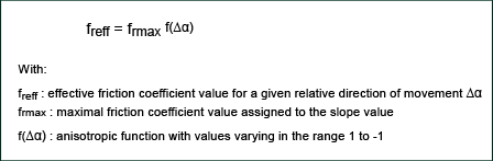
Let us illustrate the construction of an anisotropic function f() that gives a weight to the maximal friction to produce the final effective friction value. We decided to combine two different functions:

• A cosinus function cosk to model the decrease of the friction in the range 0° to 90° symmetrically from 0° to 270°. Values of the function should vary from 1 to 0 in order to produce an effective friction (freff) varying from its maximum value (frmax) to a friction value of 1 (ie. freff = frmax0 = 1). As illustrated in the next figure, an increase in the exponent k produces a faster decrease of f values with respect to the angle values Δα.
• A linear function to model the increase of the force in the range 90° to 180° and symmetrically from 270° to 180°. Values of the anisotropic function should vary from 0 to -1 in order to produce an effective friction (freff) varying from 1 to a minimum value of 1/frmax (ie. freff = 1/frmax).

The chosen simulation procedure VARCOST requires three input components:

• An image layer of maximal friction coefficient that expresses the cost distance for crossing each cell based on its maximal slope.
• An image layer of the maximal slope direction (aspect) that expresses the upward orientation of the maximal slope. In practice, most procedures that derive the maximal slope orientation from a DEM will compute it as the descending direction. It is therefore necessary to transform it into an ascending orientation that corresponds to the direction of the maximal friction.
• An anisotropic function that weight the maximal friction index according to the relative direction of movement.

Let us first assign a friction coefficient to slope values. In our example we want to express a time distance of movement. Eastman (2008) is proposing a formula transforming the slope amplitude into time of movement. This transformation produces our maximal friction coefficient layer, as illustrated in the next figure a). The corresponding ascending orientation layer is presented in b).

Based on these two image layers and with the used of the anisotropic function cos1, the time-distance image to the destination D can be generated, along with the optimal path from the origin O, as illustrated in the next figure a). Figure b) shows that the optimal path does not match the landcover distribution, simply because it was not considered during this simulation stage.

Combination of the two factors: topography and landcover
Let us now move to the ultimate stage of our simulation modeling by taking into account the simultaneous influences of the topography and the landcover on the walking movement. The procedure VARCOST allows us to combine several friction factors in order to generate a resulting friction layer and then the final time-distance image to the destination.

The next figure a) shows the resulting time-distance image with the optimal path overlayed, while figure b) illustrates the relationship of the pathway with the landcover. One can observe the added effect of the landcover friction on the optimal path: the hill is now walked from the west side and it reaches the nearest road location as fast as possible because of the low friction attached to this latter cover.