|
|
Example of CA : SLEUTH, a more complex one
Now we shortly present a CA model proposed by Clarke et al. (1998). This CA simulation model was developed to predict urban growth in the San Francisco Bay area. They have used multiple data sources: a topography map, historical maps of highway development from 1920 to 1978, existing settlement distributions and their modification over time.
The SLEUTH name is the acronym for Slope, Landuse, Exclusion, Urban, Transportation and Hillshading. These are factors controlling the urban growth process.
The control parameters of the model are allowed to self-modify, where the CA adapts to the circumstances it generates, especially, during periods of rapid growth or stagnation. The model accumulated probabilistic estimates based on Monte Carlo methods.
The next figure illustrates the four input data layers used by ![]() SLEUTH
model for simulating urban growth:
SLEUTH
model for simulating urban growth:
- Slope layer: Slope value for every cell location is derived from a DEM. It is used to determine the slope-resistance weighting.
- Excluded areas layer: Cells entirely exempt from the growth process, including oceans, lakes, and protected areas such as national parks and wetlands.
- Road layer: A binary array describing roads for a given area (read in when the time is reached) and a buffer whose width is determined by the road gravity control factor, and defining the road attractiveness for development.
- Seed layer The initial distribution of urban areas that act as growth centers. The seed layer can be any distribution taken either from an actual time period or from a hypothetical starting distribution.
 The four input data layers used by SLEUTH model for simulating urban growth (after Clarke et al.,
1997)
There are five factors that control the behaviour of the system, which are
growth control parameters in the model:
- DIFFUSION, determines the overall dispersiveness of the distribution both of single grid cells and in the movement of new settlements outward from the road network
- BREED coefficient, determines how likely a newly generated detached settlement is to start its own growth cycle
- SPREAD coefficient, controls how much outward organic expansion takes place within the system
- SLOPE-RESISTANCE, influences the probability of settlements extending upward on steep slopes
- ROAD-GRAVITY, affects the attractiveness of new settlements onto the existing road network if they fall within a given distance of a road
The values for DIFFUSION, BREED, SPREAD, and SLOPE-RESISTANCE range from
0-100, and ROAD-GRAVITY ranges from 0-20.
 Growth rules: model operation for a single cycle, a year for example (after Clarke et al., 1997)
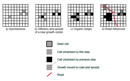
As we can see from the last figure illustrating the four growth rules, the model defines the growth rate as the sum of the four types of urban growth, which are:
- Spontaneous growth: it occurs when a randomly chosen cell falls in an area close to an already urbanised cell
- Diffusive growth: it urbanises cells that are flat and suitable for development even though they are not close enough to an urban area
- Organic or edge growth: spreads outward existing urban centers
- Road-influenced growth: promotes urbanised cells to develop along the road network
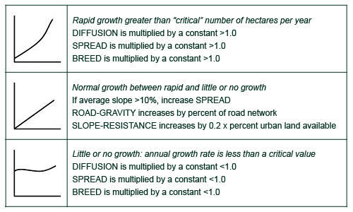
To allow the model to modify itself, a new set of rules are defined by
coupling the variables. These modification rules can be summarised in four
conditions:
- When the absolute amount of growth in any year (cycle) exceeds a critical value, the DIFFUSION, SPREAD, and BREED factors are increased by a multiplier greater than one
- When the system growth rate falls below another critical value, the DIFFUSION, SPREAD, and BREED factors are decreased by a multiplier less than one
- The ROAD-GRAVITY factor is increased as the road network expands
- The SLOPE-RESISTANCE factor is increased as the land available for development decreases
The following figure illustrates the self-modification
rules.
 Self-modification adjustments to the control parameters (after Clarke et al., 1997
The SLEUTH model was applied to the study area of Bulle (Al-Ghamdi 2008)
in order to simulate the urban development until the year 2050 according to
three ![]() scenarios of development with different levels of controlled expansion:
extreme, moderate and less control scenario.
scenarios of development with different levels of controlled expansion:
extreme, moderate and less control scenario.
This development simulation requires two main stages: the calibration stage used to train and to evaluate the model capability based on past and documented LUC for the years 1952, 1974, 1993 and 2001, followed by the prediction stage that evaluates the urban extent for future and undocumented dates.
![]() Calibration stage: five following
layers that express the input factors controlling the urban growth process were
introduced for the control years 1952, 1974, 1993 and 2001: LUC, urban extent,
road network, excluded areas and slope. During this stage a validation phase was
realised in order to estimate the capabilities to model the urban extent in 1993
and 2001. This model validation indicated a very satisfying simulation ability
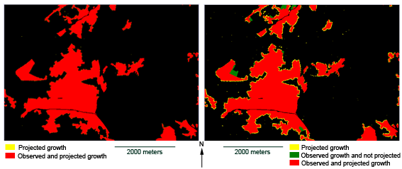
with a respective Kappa value of 0.98 and 0.95. The spatial distribution of
projected and observed urban extent for 1993 and 2001 are illustrated in the next figure.
Calibration stage: five following
layers that express the input factors controlling the urban growth process were
introduced for the control years 1952, 1974, 1993 and 2001: LUC, urban extent,
road network, excluded areas and slope. During this stage a validation phase was
realised in order to estimate the capabilities to model the urban extent in 1993
and 2001. This model validation indicated a very satisfying simulation ability
with a respective Kappa value of 0.98 and 0.95. The spatial distribution of
projected and observed urban extent for 1993 and 2001 are illustrated in the next figure.
 Projected and observed urban extent in Bulle area for 1993 and 2001 (after Al-Ghamdi, 2008)
![]() Prediction stage: mentioned above,
this simulation is aimed to predict the urban development during the period 2001
to 2050. As the SLEUTH model authorises to modify rules and controlling factors
during the iterative prediction stage, the road development plan for 2012 is
added as an input layer as is the new planned protected areas layer (next table).
Prediction stage: mentioned above,
this simulation is aimed to predict the urban development during the period 2001
to 2050. As the SLEUTH model authorises to modify rules and controlling factors
during the iterative prediction stage, the road development plan for 2012 is
added as an input layer as is the new planned protected areas layer (next table).
 Input layers used for the prediction stage (adapted from Al-Ghamdi, 2008)
Three scenarios are submitted to forecast the urban development with different levels of controlled expansion: extreme, moderate and less control scenario. In the three scenarios all land use types are excluded from urbanisation, as having a control level value of 100 (Table), except for agriculture land that is left open if it is outside existing or new planned protected areas. A zero level of exclusion is then assigned to this land use type. The difference between the three scenarios is the following:
- Extreme control scenario: all existing and new planned protected areas are given a value of 100 which excludes them from urbanisation.
- Moderate control scenario: the new planned protected areas are assigned a value of 40 for the control level, giving more chance for urbanisation with moderate limitations.
- Less control scenario: the new planned protected areas are assigned a value of 0, making them open for urbanisation, depending on rules of growth.
 Three different scenarios and level of exclusion (adapted from Al-Ghamdi, 2008)
The next slideshow illustrates the urban growth simulation during the period 2001-2050 according to the conditions and rules assigned to the three scenarios.
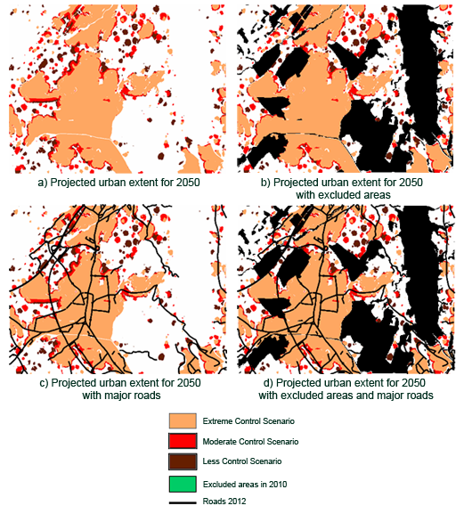
Differences between the three scenarios at the end of the simulated period are illustrated in the next figure. One can observe the influence of the control level of exclusion on the spatial growth as well as the one from the road network.
 Projected urban extent for 2050 according to the three scenarios and related with the road network and
excluded areas (adapted from Al-Ghamdi, 2008).
 EXERCISE:
From the last try to visually estimate:- The impact of the control level of exclusion on the urban extent.
- The location of new urban areas and its relation with the road network.
