Trend surface analysis

Principle

This approach is aimed to model the overall distribution of properties throughout space. It will sketch the global trend of distribution as a simplified surface.

Trend surface modelling can be applied in the following geographic information context:

• Information can be either in image (raster format) or object (vector format) form
• Properties are estimated at sampled locations, described as a set of geographical locations
• Only spatially continuous distributions can be modelled
• Properties must be quantitative, measured at cardinal level

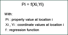
The principle of a trend surface model is a regression function that estimates the property value Pi at any location, based on the Xi,Yi coordinates of this location. The general function is:

A trend surface model is a particular case of a bivariate regression model with two independent variables, the coordinates X and Y and a dependent variable, the thematic variable P to be modelled. One can selected a linear regression function (first order) or, if the spatial distribution is more complex, a polynomial function (2nd, 3rd, …, or nth order). The modelled surface will correspond to respectively a flat oriented plane or a curved surface with an increasing number of curvatures.

In order to illustrate the principles of trend surface modelling, let’s take a phenomenon with a very obvious and observable spatial distribution: altitude. Let us suppose that we are starting our process of spatial distribution description with a sample of nn data point measurements, irregularly distributed throughout the study area to be described. One can identify 3 stages that are common to most modelling methods:

1. In the first step we select the most significant polynomial regression function that best explain the distribution of sample values. This is obtained by computing the F ratio that expresses the proportion of the total variance taken into account by the regression function. As this modelling approach is aimed to sketch the spatial distribution of properties with a continuous surface, it is recommended to limit the order of the regression function up to the fifth order. Such a surface requires 21 coefficients to be modelled. If the F ratio is not yet significant, this would mean that the distribution pattern of properties is simply too complex to be summarised with a surface function.
2. Once the regression model has been “calibrated” (i.e. estimation of function coefficient values and selection of the most appropriate function order), the regression function should be then applied to an independent set of sample points for validation purpose.
3. Finally, the selected regression function describes the considered trend surface that models the spatial distribution of properties. This function can then be used to estimate the property value at any location Xi,Yi within the study area.

The following figure illustrates the real distribution of altitude values within a study area as well as different trend surfaces modelling this distribution.

Illustration

Let us now illustrate the application of such a surface modelling process on a spatial sample of change index. Our objective is to summarise with the use of a trend surface the spatial distribution of change index values measured at different point locations in a study area. We have measured the population change of 55 localities in the district of the Sarine (in the Canton of Fribourg in Switzerland) during the period 1900-1986. The index change selected for the description of this evolution is the Normalised Difference (ND) as discussed in the section 2.1.1 of the Unit 2. Original X,Y coordinates were standardised in order to limit their unit of measurement and their influence on regression coefficient values.

Several regression functions were applied on this set of 55 points and Table summarises 3.2 their different parameters.

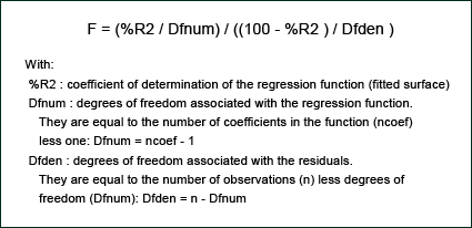
In order to test the significance of an individual trend surface model order, an F ratio should be derived from the coefficient of determination (%R²) and the degrees of freedom (Df) associated with the fitted surface and its residuals (Davis 1986) (Unwin 1975). F ratio value is computed as follows:

The F ratio values computed for each regression function order ranging from 1 to 8 are listed in the last table. They are all greater than their respective critical F value at 95 % confidence level and therefore express a significant trend. However, as our sample is made of 55 observations and as the number of coefficients increases rapidly with high function orders, it sounds reasonable to consider trend surface models up to the quintic order (order 5). From a statistical point of view there is a technique to assess the significance of contribution for selecting a higher order a lower one already significant. It is based on an F ratio value that expresses the extra contribution of an n+1 order over an n order (Davis 1986) (Unwin 1975). It is an interesting test as it compares the improvement of the fit with the increase in complexity of the fitting model. This F ratio value is computed as follows:

The following illustrates the application of the test of increasing order significance for the 8 trend surface models applied to the 55 localities of the Sarine district.

The interpretation of significance of trend functions listed before (Table) leads to the conclusion that the 8th order is the most suitable for modelling the spatial distribution as it takes into account 98.1% of the point distribution. This conclusion is confirmed by the test of significance about the additional contribution of the order 8 against the previous order (Table). However, when comparing the interpolated surface (Figure) with the modelled trend surfaces illustrated in the next figure, one can observe several strong discrepancies and artefacts generated by trend models, particularly with higher orders:

• Outside the sampled region estimated values from trend surfaces become unreal. This is known as edge effects. One should discard these regions by masking or obtain additional sample points. Such artefacts are observable from the 3rd order.
• Trend surfaces tend to fit better and better the interpolated distribution up to the 4th order. Then the distribution of values tends to be more and more different from the interpolated distribution. This discrepancy is mainly caused by the limited number of sample points compared with the rapid increase in number of coefficients attached to high order functions. Ultimately, when the number of coefficients reaches the number of observations, the trend surface will exactly fit all the observation values, but the remaining locations of this modelled surface will certainly be inconsistent.

Based on these general issues and keeping in mind that a relevant trend surface model is aimed to summarise the overall spatial distribution of properties, one should concludes that the most appropriate model for the description of this distribution could be the 4th order function. It explains around 60% of the overall variations and contains 15 coefficients, almost four times less than the number of observations.