|
|
![]()
Raster Data Compression
We can distinguish different ways of storing raster data, which basically vary in storage size and consequently in the geometric organisation of the storage. The following types of geometric elements are identified:
- Lines
- Stripes
- Tiles
- Areas (e.g. Quad-trees)
- Hierarchy of resolution
Raster data are managed easily in computers; all commonly used programming languages well support array handling. However, a raster when stored in a raw state with no compression can be extremely inefficient in terms of computer storage space.
As already said the way of improving raster space efficiency is data compression.
Illustrations and short texts are used to describe different methods of raster data storage and raster data compression techniques.
Full raster coding (no-compression)
By convention, raster data is normally stored row by row from the top left corner.
Example: The Swiss Digital elevation model (DHM25-Matrixmodell in decimeters)
In the header file are stored the following information:
- The dimension of the matrix (number of columns and rows)
- The x-coordinates of the South-West (lower left) corner
- The y-coordinates of the South-West (lower left) corner
- The cell size
- the code used for no data (i.e. missing) values
 ncols 480 nrows 450 xllcorner 878923 yllcorner 207345 cellsize 25 nodata_value -9999 6855 6855 6855 6851 6851 6837 6824 6815
                        6808 6855 6857 6858 6858 6850 6839 6826 6814 6809 6854 6863 6865 6865 6849 6840 6826 6812 6803 6853 6852 6873 6886 6886 6853
                        6822 6804 6748 6847 6848 6886 6902 6904 6855 6808 6762 6686 6850 6859 6903 6903 6881 6806 6739 6681 6615 6845 6857 6879 6856
                        6795 6706 6638 6589 6539 6801 6827 6825 6769 6670 6597 6562 6522 6497 6736 6760 6735 6661 6592 6546 6517 6492 6487 ...
PROBLEM: Big amount of data!
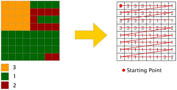
Runlength coding (lossless)
Geographical data tends to be "spatially autocorrelated", meaning that objects which are close to each other tend to have similar attributes:
"All things are related, but nearby things are more related than distant things" (Tobler 1970) Because of this principle, we expect neighboring pixels to have similar values. Therefore, instead of repeating pixel values, we can code the raster as pairs of numbers - (run length, value).
The runlength coding is a widely used compression technique for raster data. The primary data elements are pairs of values or tuples, consisting of a pixel value and a repetition count which specifies the number of pixels in the run. Data are built by reading successively row by row through the raster, creating a new tuple every time the pixel value changes or the end of the row is reached.
Describes the interior of an area by run-lengths, instead of the boundary.
In multiple attribute case there a more options available:
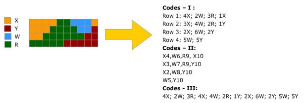
We can note in Codes - III, that if a run is not required to break at the end of each line we can compress data even further.
NOTE: run coding would be of little use for DEM data or any other type of data where neighboring pixels almost always have different values.
Chain coding (lossless)
See Rasterising vector data and the Freeman coding
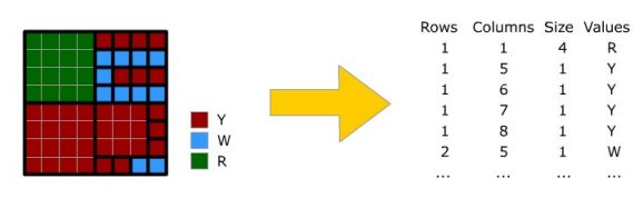
Blockwise coding (lossless)
This method is a generalization of run-length encoding to two dimensions. Instead of sequences of 0s or 1s, square blocks are counted. For each square the position, the size and, the contents of the pixels are stored.
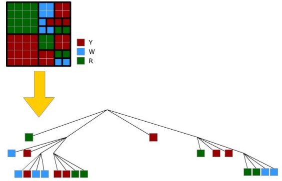
Quandtree coding (lossless)
The quadtree compression technique is the most common compression method applied to raster data. Quadtree coding stores the information by subdividing a square region into quadrants, each of which may be further subdivided in squares until the contents of the cells have the same values.
 Reading versus
Example 1:
Positioncode of 10: 3,2
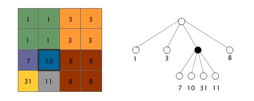
Example 2:
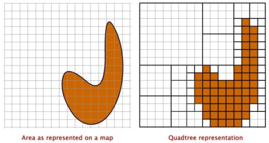
On the following figure we can see how an area is represented on a map and the corresponding quadtree representation. More information on constructing and addressing quadtrees, see Lesson "Spatial partitioning and indexing", Unit 2
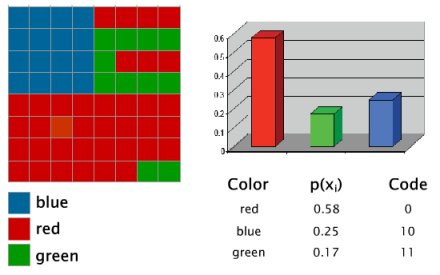
Huffman coding (lossless compression)
Huffmann coding compression technique involves preliminary analysis of the frequency of occurrence of symbols. Huffman technique creates, for each symbol, a binary data code, the length of which is inversely related to the frequency of occurrence.
LZ77 method (lossless compression)
LZ77 compression is a loss-less compression method, meaning that the values in your raster are not changed. Abraham Lempel and Jacob Ziv first introduced this compression method in 1977. The theory behind this compression method is relatively simple: when you find a match (a data value that has already been seen in the input file) instead of writing the actual value, the position and length (number of bytes) of the value is written to the output (the length and offset - where it is and how long it is).
Some image-compression methods often referred to as LZ (Lempel Ziv) and its variants such as LZW (Lempel Ziv Welch). With this method, a previous analysis of the data is not required. This makes LZ77 Method applicable to all the raster data types.
JPEG-Compression (lossy compression)
The JPEG-compression process:
- The representation of the colors in the image is converted from RGB to YCbCr, consisting of one luma component (Y), representing brightness, and two chroma components, Cb and Cr), representing color. This step is sometimes skipped.
- The resolution of the chroma data is reduced, usually by a factor of 2. This reflects the fact that the eye is less sensitive to fine color details than to fine brightness details.
- The image is split into blocks of 8×8 pixels, and for each block, each of the Y, Cb, and Cr data undergoes a discrete cosine transform (DCT). A DCT is similar to a Fourier transform in the sense that it produces a kind of spatial frequency spectrum.
- The amplitudes of the frequency components are quantized. Human vision is much more sensitive to small variations in color or brightness over large areas than to the strength of high-frequency brightness variations. Therefore, the magnitudes of the high-frequency components are stored with a lower accuracy than the low-frequency components. The quality setting of the encoder (for example 50 or 95 on a scale of 0–100 in the Independent JPEG Group's library) affects to what extent the resolution of each frequency component is reduced. If an excessively low quality setting is used, the high-frequency components are discarded altogether.
- The resulting data for all 8×8 blocks is further compressed with a loss-less algorithm, a variant of Huffman encoding.

JPEG-Compression (left to right: decreasing quality setting results in a 8x8 block generation of pixels)
Text and graphic from: Wikipedia 2010
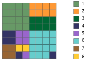
Example of runlength coding
In the following example, we can see the difference in data storing, between an uncompressed raster file and a compressed one.
 Full raster coding 256 values Full raster coding 256 values |
 runlength coding 132 values runlength coding 132 values |
Proof your knowledge
Compress the following raster file with the compression techniques that you have learnt in this unit.
How much space is needed for storage, if we assume that bytes (8 bits) can be used to store the data values?
|
|
|
|