|
|
![]()
Methods for time series
Evolution of thematic properties throughout time can be described in
greater details by measuring the property of individual observation (each
spatial feature) at numerous intervals of time during the considered period.
Time intervals can be either regular or irregular. However many methods require
a same regular interval that is common to all observations in order to allow
comparison. For each observation this sequence of property values is called a
![]() time series. Time series collected for a
set of observations can be structured as a two-dimensional data table as
illustrated below.
time series. Time series collected for a
set of observations can be structured as a two-dimensional data table as
illustrated below.
 Change in number of inhabitant during the period 1900 – 1990 with an interval of 10 years
 Change in political majority during the period 1900 – 1990 with an interval of 10 years
Individual property change:
The objective is again to summarise the individual time change behaviour with a single index value. This can be done by the use of typical statistical descriptors (central tendency and dispersion) or by modelling the trend in change.
Summary statistics
With a simple statistical descriptor some
aspects of the individual change behaviour can be described such as its central
tendency, its variability or a combination of both. Depending on the nature of
data analysed (qualitative or quantitative), the following statistical
descriptors are applied to summarise the change:
- For qualitative data time series: the mode and the diversity
- For quantitative data time series: the mean or the median, the standard deviation or the interquartile, the coefficient of variation and the range.
Let us illustrate the use of statistical descriptors for summarising the
time change behaviour of features described in the two tables
above.
The time series describing the political majority during the period 1900-1990 for 9 municipalities are qualitative data measured at nominal level, therefore two indicators can be applied, the mode for deriving their central tendency and the diversity for their dispersion as expressed below
 Statistical descriptors applied to summarise the change in number of inhabitant during the period 1900 – 1990
EXERCISE
- Municipalities A, F and H have the same modal value, In what respect their diversity value contributes to express a difference in change behaviour?
- What interpretation can be made about the municipality E based on its modal property (bi-modality) and its diversity?
The time series describing the number of inhabitant during the period 1900-1990 for 9 municipalities are quantitative data measured at cardinal level, therefore six different indicators can be applied for deriving their central tendency and dispersion
 Statistical descriptors applied to summarise the change in number of inhabitant during the period 1900 – 1990
Change trend modelling
The objective of such modelling is to
summarise with a single index value the time change behaviour of each
observation. Such a constraint limits the panel of functions to very simple
ones. Two models expressing the trend of
change could be retained: the ![]() linear
regression and the
linear
regression and the ![]() allometric
function. More precisely, a single coefficient for each model
will be retained in order to express the change trend.
allometric
function. More precisely, a single coefficient for each model
will be retained in order to express the change trend.
The trend of a linear model can be summarised as the slope coefficient b of the linear regression function Y = a + b X. In the case of time change modelling, the variable X is the time and Y is the considered phenomenon. In a growth process, as in many change processes, the property values of a phenomenon do not often increase in a linear manner with respect to time. Time series values can be transformed by the application of a logarithmic (log) or a square root (sqrt) function in order to compensate for this non linear increase. As the linear trend coefficient should describe best the change behaviour, the analyst should apply to the original time series values the most efficient transformation to compensate for this non linear behaviour.
This linear model can then take the following forms:
- For a linear increase in the original time series values: Y = a + b X
- For a non linear increase in the
original time series values:
logY = a + b X or
sqrtY = a + b X
with X as the time variable and Y the considered phenomenon
The principle of modelling the evolution trend is illustrated below. From the three time series illustrating property change
of three
hypothetical situations throughout time, one can observe that the slope
coefficient b of a linear regression
function is capable to summarise the evolution pattern of each
series.
 Modelling the behaviour of 3 time series with the use of their respective slope coefficient b of the linear regression
Assuming the adjustment of the linear trend is satisfying for each
individual time series, then b coefficient can be interpreted as the growth
rate. The coefficient value expresses the strength of change, a positive value
indicates an increase as a negative value suggests a decrease throughout the
period of time. However the comparison between coefficient values is limited due
to the influence of the size of values on the trend coefficient b. There are
several techniques proposed to standardise this coefficient for comparison
purposes, but an efficient way to perform comparison is the use of an allometric
function.![]() Allometry is a model developed in the context of biology. It
attempts to describe the relative growth of a body part with respect to the
growth of the whole body (organism). With the rise of the systemic approach in
sciences, this concept of relative growth was then associated with principles of
interactions between a set and its subsets (parts). Let us start with a
definition: “Allometry: the relative growth of a part
in relation to an entire organism or to a standard” (Anonymous). Thus one can summarise the relative growth of individual
features with respect to the growth of the whole, in our case the set of
considered features.
Allometry is a model developed in the context of biology. It
attempts to describe the relative growth of a body part with respect to the
growth of the whole body (organism). With the rise of the systemic approach in
sciences, this concept of relative growth was then associated with principles of
interactions between a set and its subsets (parts). Let us start with a
definition: “Allometry: the relative growth of a part
in relation to an entire organism or to a standard” (Anonymous). Thus one can summarise the relative growth of individual
features with respect to the growth of the whole, in our case the set of
considered features.
The allometric law is defined as follow:
- In original form:
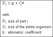
- In linear form:
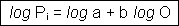
In this linear form the allometric coefficient b -which is also the slope coefficient of the linear regression model- can be interpreted as follow:
 can be interpreted as the relative growth rate of the corresponding feature.") Modelling the growth of 3 features throughout time with respect to the growth of a whole. The b allometric coefficient (slope)
can be interpreted as the relative growth rate of the corresponding feature.
Modelling the growth of 3 features throughout time with respect to the growth of a whole. The b allometric coefficient (slope)
can be interpreted as the relative growth rate of the corresponding feature.The b change index provides information about the type and the rate of relative change of individual features. Comparison between bi index values is then made possible, as well as mapping their spatial distribution within the study area.
Illustration
Let us now illustrate the use of regression slope coefficient and allometric coefficient to summarise the evolution of telephone subscriptions in each municipality between 1900 and 1990. We know that individual evolution is influenced not only by factors governing the diffusion of innovation, but also by the increase of potential subscribers (households) within the considered period of time.
 Change in number of telephone subscription during the period 1900 – 1990 with an interval of 10 years
The growth trend of each municipality during this period of time can be
first summarised with the use of the slope coefficient
b. As growth rates are not linear (Figure) it is necessary
to apply a transformation to original data. In this case the most adequate
transformation is the square root function (Sqrt). Transformed data can now be
fitted with a linear regression model:
sqrtY = a + b X
with X as the time variable and Y the number of
telephone subscription for each municipality
 Diagram showing the evolution of number of telephone subscription during the period 1900-1990 for each municipality. It clearly
illustrates the non linear progression for all features.
Diagram showing the evolution of number of telephone subscription during the period 1900-1990 for each municipality. It clearly
illustrates the non linear progression for all features. Diagram showing the effect of the square root transformation applied to original data illustrated in the previous figure.
Individual growth rate is summarised in the following table with the use of their respective b slope coefficient. Because this process has started only around 1920 for most municipalities the slope coefficient was calculated also for the period 1920-1990.
 Slope coefficients calculated for the whole period 1900-1990 as well as for the period 1920-1990 on square root transformed
data.
Slope coefficients calculated for the whole period 1900-1990 as well as for the period 1920-1990 on square root transformed
data.Several comments can be made about these coefficients:
- The slope coefficient expresses the absolute amount of subscription increase during the considered period. This is confirmed by the strong correlation between the number of telephone subscription in 1990 and the slope coefficient value.
- Such index values should be interpreted as a global rate of increase during the whole period. Nothing is said about the relative dynamics among features.
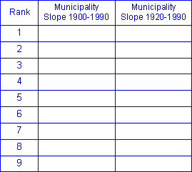
EXERCISE
Compare the change trend index (slope coefficient values) for the 2 considered periods 1900-1990 and 1920-1990:
- What general considerations can be made?
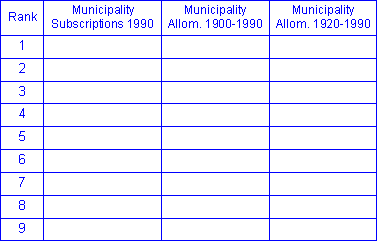
- In the following Table, rank municipalities according to their respective slope values for the two periods. Compare and comment on rank changes:
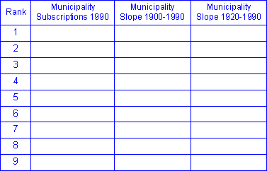
Rank and compare the number of telephone subscriptions in 1990 (Table) and the slope values for the two periods:
Let us now illustrate the contribution of the allometric coefficient as a change index. As you remember the linear form of the allometric function is the following:
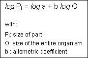
The allometric coefficient is therefore the slope coefficient b of the
function relating the growth of a part Pi (here the Municipality i) with the one of the whole O (here
the District).
Individual relative growth rate is summarised below with the use of their respective b
allometric coefficient. Because this process has started only around 1920 for
most municipalities the allometric coefficient was calculated also for the
period 1920-1990.
 Allometric coefficients calculated for the whole period 1900-1990 as well as for the period 1920-1990.
Several comments can be made about these coefficients:
- The allometric coefficient expresses the relative growth rate of each municipality during the considered period. This is confirmed by the coefficient value of 1 for the district which corresponds to the entire set of municipalities.
- The sub-period 1920-1990 expresses best the relative growth rates, as most of municipalities have started only from 1920.
- For the period 1920-1990 there are two cases of positive allometry and seven cases of negative allometry. However municipality H is very close to isometry. Municipality B has the highest coefficient value while the municipality I has from far the lowest.
EXERCISE
Compare the change index (allometric coefficient values) for the 2 considered periods 1900-1990 and 1920-1990:
- What general considerations can be made?
- In the following Table, rank municipalities according to their respective coefficient values for the two periods. Compare and comment on rank changes:
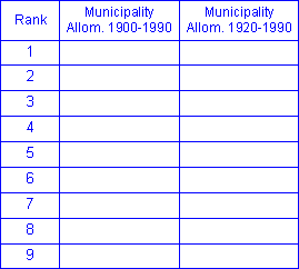
Rank and compare the number of telephone subscriptions in 1990 (Table) and the allometric coefficient values for the two periods:
Then compare the observations made for the slope coefficients and the allometric coefficients.
Global property change:
Another way to summarise the behaviour of individual features throughout
time is to synthesise the time dimension variables into synthetic component.
Finally index values will be attached to each feature (component scores) but
they are derived from a global analysis of the whole set of features and time
variables. The objective is again to summarise the individual time change
behaviour with a couple index values. Such a transformation is called ![]() Principal
component transformation or analysis (PCA), it produces principal component scores for each
feature.
Principal
component transformation or analysis (PCA), it produces principal component scores for each
feature.
Standardised principal component scores
One can read the content of the following table as a set of time series describing the change in number of inhabitant during a period of time for the nine considered municipalities (row direction reading). This table structure can be approached from the column direction as well. This time census dates are interpreted as time variables. Each of them describes the number of inhabitant in the nine municipalities at a specific date. As properties change smoothly from a census date to another, one can expect a fairly high degree of correlation between time variables. Therefore it seems reasonable to synthesise this set of variables (here 10 dates or 10 variables) into a few number of relevant components.
 Change in number of inhabitant during the period 1900 – 1990 with an interval of 10 years. Features are the nine municipalities
and variables are the 10 census dates.
Change in number of inhabitant during the period 1900 – 1990 with an interval of 10 years. Features are the nine municipalities
and variables are the 10 census dates.This high degree of correlation is illustrated by the corresponding correlation matrix in the next table. One can observe the following:
- The strongest correlation takes place between a date and its preceding or its next one.
- The degree of correlation decreases with the distancing of census dates.
- The variable 1960 has the overall highest degree of correlation with all other variables.
 Correlation matrix for the ten time variables. It shows the strong degree of correlation between variables.
In order to remove the undesirable scale effect, variables should be standardised prior to the component transformation.
The principal
component transformation produces two significant components, summing up 99.5%
of the total variance:
- component 1 (PC1): 85.3% of variance
- component 2 (PC2): 14.2% of variance
The contribution of original variables to the two retained principal components is expressed by their respective weights in the component matrix. The figure below illustrates this contribution. One can observe the following:
- Years 1900 to 1960 have a strong influence on the component 1 (1960 with the strongest), while 1970 to 1990 have a lower one (1990 with the weakest). All weights are positive.
- For the component 2 weights range from negative to positive. Once again the 2 groups of variables can be identified. The order of weights almost follows the sequence of years.
 Weight of variables on the two principal components.
EXERCISE
Assign a name to the two principal components that describes best their content:
- Component 1: (relative population size during the period)
- Component 2: (recent growth rate versus early one)
Now let’s consider the properties of the 9 municipalities for the two principal components. Their respective score values can be plotted for identification of groups with similar evolution behaviour. From the next figure three groups of features can be identified:
- Group 1: made of a single outsider B
- Group 2: made of municipalities F and H. Their two index values are positive
- Group 3: the largest group that includes the 6 remaining municipalities. Index values (scores) for both components are almost negative. However, municipality G is slightly away from other members of this group, with a positive index value for the first component.
 Score values of the 9 municipalities for the two principal components.
Interpretation of score values as a global behaviour index is made
possible by comparing with the diagram of population change during this period
of time.
Score values of the 9 municipalities for the two principal components.
Interpretation of score values as a global behaviour index is made
possible by comparing with the diagram of population change during this period
of time.
 Population change for the 9 municipalities during the period 1900-1990.
EXERCISE
Compare curve shapes of municipalities from the last diagram with their respective score values plotted in the last figure. Characterise and comment on the proposed grouping:
- Group 1:
- Group 2:
- Group 3:
|
|
|
|