Time as a sequence of events (with regular intervals)

In this context the behaviour of each feature is expressed throughout the considered period of time as a succession of properties or events measured during an interval of time ti. In order to illustrate several of the methods discussed in this Section, let us take a simple example. We are interested in the analysis of car accidents occurring in the municipalities of our study area during a period of 3 years (1988 to 1990). The considered phenomenon is then the frequency of car accidents reported to the police during each month in this period in each of the municipalities. From these reports a time series made of 36 monthly counts was then produced. It describes the behaviour or the profile of each municipality during this 3 years period of time. Let us now concentrate on the two municipalities E and I with their respective time series listed in the table below.

The behaviour of individual features can be described and analysed in many different ways with various considerations about the time dimension:

• In which way properties change during the period of time?
• Is there any regular scheme of properties?
• How this individual behaviour compare with a reference behaviour?
• Can this behaviour be generalised and modelled?

Let us first briefly summarised the overall property distribution for the two municipalities during this 3 years period of time. Descriptive statistics indices provide us with basic characteristics about property values present in each time series. Numerical indices listed in the table below indicate that the total number of car accidents is 73 for both municipalities and that their respective mode, mean, median, and standard deviation are identical. Their histogram shown in the next figure is confirming an identical distribution of property values during this period of time.

Furthermore the two distributions follow almost perfectly a Poisson distribution with a mean value of 2.03. A Chi-square test as well as a Kolmogorov-Smirnov test indicate that the differences in frequency distribution between the Poisson distribution and the two observed distributions are strongly not significant. This indicates that during the period of 36 months the frequency of monthly car accidents do not depart from a random distribution having a mean value of 2.03. In other words, there is no individual factor in both municipalities that strongly affects the variations in the frequency of monthly car accidents. The following table shows the comparison between a Poisson frequency distribution and the two observed distributions.

Can we then conclude to an identical behaviour of this phenomenon in the two municipalities during this 3 years period? Let us observe the contribution of the time dimension for an in depth analysis of individual feature behaviour.

Runs test:

Let us analyse the sequence of properties occurring within a time series. Our interest is in the succession pattern of property values. At ordinal or cardinal level property values can increase or decrease regularly or can present a variety of change patterns. For a measurement at nominal level our interest is in the change of a category to another one.

A runs test operates at nominal level and more precisely for a binary variable with only two possible properties or states. One should therefore accommodate the original time series by a transformation grouping all possible properties into two states 0 and 1.

A runs test aims to compare the observed time series with a random sequence of states. It is used to test for randomness of occurrence. Let us consider the experiment of tossing a coin and the time series as the result of 16 successive tosses. Assuming an equal probability of 0.5 for obtaining a head (H) or a tail (T) for each toss, a large variety of sequences combining 8 heads and 8 tails can be obtained. The two following sequences illustrates extreme situations that unlikely occur at random:
- Grouped sequence: H H H H H H H H T T T T T T T T
- Regular alternation: H T H T H T H T H T H T H T H T

The succession of states corresponds to a specific pattern of the considered time series. In order to describe the pattern the full sequence is subdivided into runs. A Run is defined as an uninterrupted succession of the same state. In our previous example only 2 runs can be identified for the grouped sequence as 16 runs occur in the regular alternation sequence. For a random sequence the number of runs should be situated between these two extreme values.

It is admitted, when the number of occurrence n₁ and n₂ for each of the two states exceeds ten, that the distribution of random arrangement of two states within a sequence can be approximated by a normal distribution with an expected mean Û and its variance σ²û defined as follow:

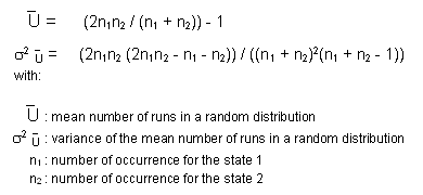
We can then applied a Z test to compare the observed number of runs U with the expected one from a random sequence:

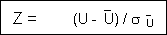
The null hypothesis and its alternative are:

With a 5% level of confidence the Z value should be less than –1.96 or greater than 1.96 to reject H0 and then to conclude that number of runs in the sequence is significantly different from the one in a random sequence.

Let us now look at the application of the Runs test to our illustrative examples: first the succession of mayor gender for municipalities E and F and then the sequence of monthly car accidents in municipalities E and I.

The first variable “gender of the municipality mayor” illustrate a series of binary properties, female or male. The next table lists the sequence for each municipality between 1900 and 1990. Thus the original values can be used to identify the number of runs in each sequence for the municipalities E and F. The two sequences are the following, with 1 for Female and 2 for Male:
Municipality E: 2 2 2 2 2 2 2 1 1 1
Municipality F: 2 2 1 1 2 1 2 2 1 2

For the municipality E we can count only 2 runs and calculate a value Z = -2.209. Thus the null hypothesis of a random sequence can be rejected with a level of confidence of 5% as the Z value is less than –1.96. The presence of only two runs within the sequence has only very little chance to result from a random arrangement; therefore there are certainly specific factors that contribute to this situation. On the contrary the sequence for municipality F cannot be considered as significantly different from a random sequence. It contains 7 runs and its Z value 0.492 lies within the critical region (± 1.96).

We are now concerned with the description of time series related with the number of monthly car accidents in municipalities E and I (Table). We would like to analyse the succession of monthly accidents with respect to the central tendency of the considered time series. Let us then group monthly frequencies into two categories: category 0 containing months with frequencies below the mean value (i.e. 2.03 for both time series) and category 1 including months with frequencies above it.

The following table summarises results for the grouping procedure and for the runs test applied to the time series of municipalities E and I. While both time series have the same number of cases below and above the mean value, their sequential distribution within the same period of time is obviously and significantly different. The number of runs for time series E is significantly less than a random time series distribution, but this is not true for the time series I with a Z value that belongs to the interval of confidence of 5%.

The graphical representation of the two series in next figure illustrates the differences of time distribution that is pointed out by the runs test. It shows that time series I crosses the threshold value almost twice as much as time series E. One can notice the strong influence of the threshold value on the number of produced runs.

When transforming the original time series from an ordinal or cardinal level down to the nominal binary level, different criteria can be applied to determine the threshold value for grouping into two categories:

• Differentiating between values below or above some threshold (ie. the central tendency as illustrated)
• Differentiating between “increasing” and “decreasing” situations.

It should be noted that the runs test reports only on the number of runs within the sequence, there is no specific information about the length of each run.

Markov chains:

You will recall from the section Global Property Change that we were interested in the summary of change within a period of time with the use of only two time markers or limits. Transition matrices were used to describe the global change of political majority in the nine municipalities between 1900 and 1990. We have then introduced the notions of transition frequency matrix, transition relative frequency matrix and transition proportion matrix. This was applied to summarise the overall change trend within the set of municipalities.

We would like now to analyse the succession of states within a single time series in order to evaluate the probability of transition from one state to another. This refers to a transition probability matrix. Furthermore this matrix expresses the probability that a state A will follow a state B, provided B occurs. This is called conditional probabilities that are contained in the transition probability matrix.

In complement to the evaluation of global probability of occurrence from any state to any state based on the analysis of the transition matrix, the construction of Markov chains offers further investigations on the sequence of state changes:

• to estimate the probability of occurrence from any original state to any final state after a specific sequence of n steps,
• to estimate the probability of occurrence of each intermediate state in a specific sequence of n steps,
• to compare transition probabilities for the observed sequence with some reference models: deterministic, random, uniform, …

Let suppose a time series composed of 64 observations regularly distributed within a period of time as illustrated in the following table.

There are three possible states labelled A, B and C. As seen before, a 3x3 transition frequency matrix can be constructed showing the number of times a given state is succeeded by another.

The measured time series contains 64 observations, so there are (n-1) = 63 transitions. Note that the rows and columns totals will be the same, provided the sequence begins and ends with the same state otherwise two rows and two columns will differ by one.
It is then possible to derive the transition relative frequency matrix and the transition proportion matrix (as expressed in the two following tables)

Comparison with a reference sequence
An observed sequence can then be compared with a reference sequence based on their transition frequency matrix (counts or relative frequency). The reference series can be either a theoretical model (deterministic, random, uniform, …) or another observed sequence. One can use a Chi-squared test to determine if the observed series is significantly different from the reference.

Analysis of the succession of changes
A sequence in which the state at one point is partially dependent on the preceding state is called Markov chains (named after the Russian statistician, A.A. Markov). A sequence having the Markov property is intermediate between deterministic sequences and completely random sequences. “In theory, the probable state of a Markov system at any future time can be predicted from knowledge of the present state” (Davis 1986).
From the transition proportion matrix (Table) it is then possible to evaluate the probability of occurrence of any state from any original state after a specific number of time step in the sequence, assuming the relative frequency distribution from the observed sequence is representative from the overall behaviour of the phenomenon. In other words, one assumes that the relative frequencies correspond to the probabilities from the parent population. When handling simple situations with few states and very few steps, it is possible to obtain such probability of occurrence by an experimental approach, but a more general solution can be found with the combination of conditional probabilities.
Let us take a simple situation to illustrate these two approaches. We would like to estimate the probability of ending with the state A when starting with this state A in a two transitions sequence (a sequence with two steps), based on the observed sequence (Table).
Experimentally we can start from the transition proportion matrix (Table) to construct a diagram of all possible two steps sequences starting from the state A with their corresponding conditional probabilities.
Diagram showing all possible sequences of two steps starting from state A with their corresponding conditional probabilities From this diagram one can identify three corresponding sequences:

The probability of occurrence for each sequence is obtained as following:

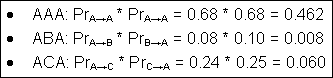
Then the overall probability of ending with the state A when starting with this state A in a two transitions sequence is:

It then become tedious to compute experimentally all other possible sequences of combination of three different states. Furthermore when the number of states and the number of steps increase, this becomes simply impossible to achieve. This can be obtained with ease by matrix algebra.

In order to derive the probability of obtaining any i state from any original state after n steps, the resulting probability matrix is simply the original “transition proportion matrix” called probability matrix [P] powered to the number of step n: [P]ⁿ.

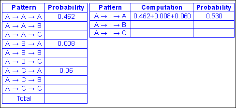
When applied to our above example, the resulting probability matrix [P]² illustrated in the following table shows not only the experimentally resulting probability Pr_A→i→A but also probabilities for all other combinations.

It is interesting to observe that when the number of step becomes important the rows tend to become similar. This indicates that the influence of the original states diminishes with time; it is the expression of the “persistence of memory” in a Markov process, as illustrated below.

Time dependency:

From our everyday experience we are aware that the current property of a phenomenon is related with its property a moment before as well as a moment after. This influence is known as the time dependency. If we consider the physical phenomenon air temperature, we can feel that temperature properties are changing throughout days, months and seasons but in a more or less continuously manner. We can then express the rate of change of temperature within a specific period of time. Many physical, but also social and economical phenomena present such a continuous temporal change of properties, although they can include some more or less abrupt discontinuities from time to time. One analytic interest is to describe this rate of change that expresses somehow the strength and duration (length) of the time dependency. At the opposite one can found phenomena with no temporal continuity, they are called chaotic as properties are distributed like randomly throughout time. This influence observed in the time dimension can be extended to the geometrical or spatial dimension. The most obvious example is certainly the distribution of elevation along a profile. Elevation properties vary continuously from a location to the contiguous one. This is known as the spatial dependency of the phenomenon. The rate of change and the duration of the dependency can be also estimated in this geometrical dimension.

Another interesting property of change is certainly the identification of periodicity or sequences within a period of time. When the periodicity is obvious we are then observing a cyclic phenomenon. Perfect cyclic phenomena are very rare in the reality and this property depends on the time scale considered. The air temperature illustrates once again a cyclic phenomenon with regular periodicities: daily, seasonally, annually, … Although such repetitive pattern is not perfect, it is then possible to identify similar patterns within a considered period of time.

As in the context of time series the description of property change is expressed by regular measures throughout the time period, the indication of similarity can be estimated by a coefficient of correlation. One can then compare the property of each step in the period of time with the one from the next and the following steps successively. This is known as the auto-correlation technique. Practically the correlation coefficient is computed between a time series and itself with successive offsets between the time positions (intervals). The amount of offset between the two time series is called a lag. When the two series are correlated with no offset, the lag equals 0 and of course the correlation is perfect and without any interest. Assuming a time series made of n positions (measures, steps), one can potentially compute correlation with different offsets varying from 0 to n-1 lags. However for the significance of the correlation coefficient the number of compared pairs must be sufficient. This number depends on the size n of the time series and on the lag value. Usually the recommended maximum number of lags is about n/4

The series of correlation coefficients computed for each successive lag can be represented graphically as a correlogramme. It can be interpreted to evaluate the duration and the strength of the dependency as well as the presence and the duration of periodicities.

As the measure of correlation should be adapted to the level of measurement of the time series, one can imagine to use the three typical correlation indicators adapted to each level:

• At cardinal level: correlation coefficient of Pearson (or Spearman for detecting non linear correlations)
• At ordinal level: correlation coefficient of Spearman
• At nominal level: association coefficient of Cramer (Cramer’s V).

To test the significance of the similarity between the two series at each specific lag, the computed correlation value is compared with the one obtained from random sequence of values.

However, in practice we tend to limit the content of time series to two situations: nominal level for categories and cardinal level for continuous values. Specific auto-correlation indicators are developed: the linear auto-correlation coefficient for the cardinal level and the match ratio for a measure of auto-association at the nominal level.

Auto-correlation:
The linear correlation coefficient calculated at each lag L is the following:

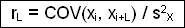
Regardless of the number of pairs considered at each lag value, the denominator of the ratio rL corresponds to the variance of the whole time series. When L=0 then the correlation coefficient corresponds to the linear correlation coefficient of Pearson. Thus r_L value varies between –1 and +1 and can be interpreted as the Pearson’s coefficient:
A + sign indicates a direct correlation as a – sign indicates an inverse correlation
The strength of the correlation varies between 0 for no correlation to 1 for a perfect one.

The significance level of the correlation at each lag L can be estimated using the normal standardised probability distribution z with:

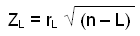
We can then plot the successive values in a diagramme of auto-correlation called correlogramme. Its interpretation will reveal the structure of the analysed time-series in terms of time influence decrease (rate of change) and presence of periodicities (cycles).

Let us now briefly illustrate this technique with the two time-series on the frequency of car accidents for municipalities E and I presented here. As each series is composed of 36 observations, the recommended maximum number of lags is about 9 (or n/4), however this number will be extended to 19, about the half of the series length, in order to better visualise possible cycles.

Auto-association:
At nominal level properties expressed by numerical values have no hierarchical meaning. Thus the only possible element of comparison between pairs of value is the “matching state”. Within each compared pairs, property values are either identical (match) or different (mismatch). Thus an index of similarity can be developed for measuring at each successive overlap position (match position, lag) the degree of similarity or association. Intuitively we can imagine this index as a ratio between the number of matching states and the number of comparisons:

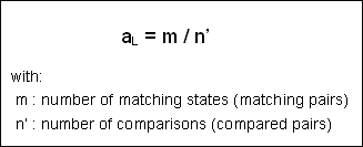
Regardless of the number of compared pairs that change according to the lag value, this ratio varies between 1 and 0. A value of 1 indicates a perfect similarity or association as 0 indicates no association at all.

Similarly to the correlogramme, one can then plot the successive values in a diagramme of auto-association called associatogramme. Its interpretation will principally reveal the presence of periodicities (cycles) within the structure of the analysed time-series.

The significance level of the association at each lag L can be estimated using either a Chi-square test or an approximation of the binomial distribution (Davis 1986, p. 251). With a Chi-square test we compute a normalised difference between the number of observed matches in the sequence and the number of matches in a random sequence. This corresponds to the binomial probability of a given number of matches occurring when a random sequence is compared to itself. It is given by:

Once the probability of a match (Pr) for a random distribution is computed, one can deduce the probability of a mismatch Q as:

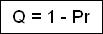
We can now estimate the number of matches (E) and mismatches (E’) occurring in a random sequence:

It should be noted that the number of comparisons n’ expresses the length of the effective compared sequence (overlapped segment) and therefore varies according to the offset (lag value).

We now have described all the components for the computation of the Chi-square value at each lag L:

Assuming this Χ² test statistic has 1 degree of freedom, one can determine the significance of the association index value for each lag L. A Yates’ correction factor can be applied to this statistic if the number of expected matches is small as with a reduced overlapping segment (Davis 1986, p. 250).

Let us now again briefly illustrate this technique with the time-series on the change in political majority during the period 1900-1990 for the municipality E presented in section Methods for Time Series. The series is composed of 10 observations, with 4 different properties (categories). Applying the previous rule, considered lag range from 0 to 3 for the computation of the index of similarity a_L . We have included lag 0 to illustrate the situation of comparing the time series with itself without any offset. The table below shows the pair comparison for the considered lag range.

Steps of the procedure are the following:

1. Computation of the index of similarity value a_L for lag 0 to lag 3
   a_L values can now being computed as the ratio of the number of matching pairs divided by the number of compared pairs. The detailed computation is shown below.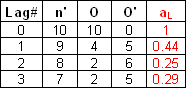
2. Computation of the probability of matches in a random sequence
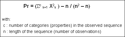
   We first have to calculate (Σ^c_k=1 Χ²_k ) in the above formula: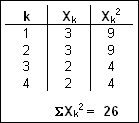
   
   Finally Pr and Q have the following values for a sequence of 10 observations with 4 different properties:
   • Pr = (26 – 10) / (100 – 10) = 16 / 90 = 0.18
   • Q = 1 – 0.18 = 0.82
3. Computation of the Chi-square value for each lag L
   The table below details the computation of each Chi-square value: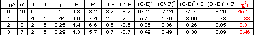
4. Test of significance of Chi-square value for each lag L
   With a degree of freedom ν = 1 and a confidence level of 95%, the critical Chi-square value is 3.84.
   We can then conclude that Chi-square values for lags 0 and 1 are significant as they are not for lags 2 and 3. In other words the auto-association is significantly different from a random sequence for lags 0 and 1 but not for lags 2 and 3. Its time dependency decreases rapidly but the short length of this illustrative series does not permit to observe the possible presence of change cycles. It is therefore not relevant to build up an associatogramme.