Cross-correlation

We know that the correlation techniques express the amount of synchronised change between two phenomena or variables. When applied to the time dimension one can compare property changes of an individual feature for two different variables during the same period of time. Similarly it is possible to compare the behaviour change of two different features for the same variable. This is obtained by comparing two time-series. For both situations one expects to discover a significant similarity between the two variables or the two features during the considered period of time. The hypothesis of a significant relationship between features or variables can be validated only when change is synchronised within the considered period of time. Let us suppose that two phenomena are strongly correlated, but with a time-lag between them or that two features are influenced by a same factor but with a different time response and speed. Thus a simple correlation procedure that compares the two time-series values on a date-by-date basis will indicate a very low degree of correlation. We have seen in section Time dependency a technique called auto-correlation that is capable of comparing a time-series with itself with different time-lag values. One can then imagine to apply this principle for the comparison of two variables or two features shifted forward or backward. This can be performed with a technique called cross-correlation. The context of use is slightly different and more complex than the one of the auto-correlation:

• The length of the two compared time-series might be different.
• To fully investigate possible shifts in time between the two series one should consider not only positive time-lags but also those ones negative. We will then prefer the term of match positions rather than lags to describe the successive comparisons.
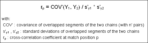
• The equation for cross-correlation differs slightly from the auto-correlation index, but still refers to the Pearson linear correlation coefficient. If the two series are called Y₁ and Y₂ and the number of compared pairs (overlapped positions) between the two chains at the match position p is designated as n’, then the equation can be written as follow:
  
• The significance of the cross-correlation coefficient at each match position m can be evaluated by an approximate test derived from a test developed for the correlation coefficient:
  
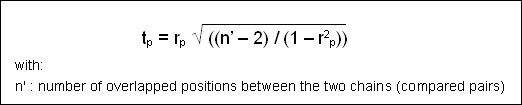
  The degrees of freedom ν equals n’-2 and the null hypothesis states that the cross-correlation is not significantly different from zero.

Let us return to the evolution of the number of car accidents in municipalities E and I during the period of 26 months. This figure illustrates the regularity of car accidents peak every 6 months for municipality I and every 12 months for municipality E. When comparing their evolution pattern with cross-correlation technique, one can expect to observe the following:

• There is no time-shift between peaks for the two municipalities as they match every month of July.
• Around February the difference between the two municipalities is the strongest.
• Cycle length is about 6 and 12 months for municipality I and E respectively.