|
|
![]()
Cross-association
The ![]() cross-association is the alternative technique for the pairwise comparison of change
pattern between either two different features or two variables of the same
feature, when the level of measurement is nominal (qualitative data). The
comparison process between the two time-series is similar to the
cross-correlation technique, but the measure of correspondence (degree of
correspondence) at each match position is the index of similarity. It is the
same ratio as the
cross-association is the alternative technique for the pairwise comparison of change
pattern between either two different features or two variables of the same
feature, when the level of measurement is nominal (qualitative data). The
comparison process between the two time-series is similar to the
cross-correlation technique, but the measure of correspondence (degree of
correspondence) at each match position is the index of similarity. It is the
same ratio as the ![]() index of similarity
aL computed for the
auto-association, but this time it is called ap as match position can be negative or positive:
index of similarity
aL computed for the
auto-association, but this time it is called ap as match position can be negative or positive:
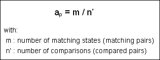
Again the ratio range between 0 and 1, expressing the strength of similarity between the two segments compared at match position m. Successive values can be plotted in an associatogramme to identify match positions with a high degree of similarity and the to interpret the related shifts in time.
The significance level of the association at each match position m can again be estimated using either a Chi-square test or an approximation of the binomial distribution. Just like for the auto-association case, with a Chi-square test we compute a normalised difference between the number of observed matches in the segment of sequences and the number of matches in a random sequence. But in this context it corresponds to the binomial probability of a given number of matches occurring when two random sequences are compared. It is given by:
Then the following steps are identical to those applied for auto-association index evaluation. Once the probability of a match (Pr) for a random distribution is computed, one can deduce the probability of a mismatch Q as:

We can now estimate the number of matches (E) and mismatches (E’) occurring in a random sequence:
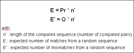
It should be noted that the number of comparisons n’ expresses the length of the effective compared sequence (overlapped segment) and therefore varies according to the match position.
We now have described all the components for the computation of the Chi-square value at each match position p:
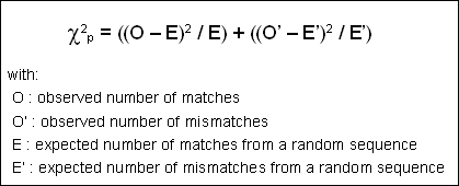
Assuming this χ2 test statistic has 1 degree of freedom, one can determine the significance of the association index value for each match position p.
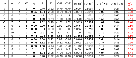
Let us illustrate this procedure of cross-association with the comparison of political majority change between municipalities A and E during the period 1900-1990 (Table). The two series being similar in size –same period- but describing two different features, comparison should be applied at both negative and positive shifted positions as illustrated in the following table.
 Comparison of political majority change between municipalities A and E. Pairs compared for match positions ranging from -7
to +7, compared segments are in bold.
Comparison of political majority change between municipalities A and E. Pairs compared for match positions ranging from -7
to +7, compared segments are in bold.Steps of the procedure are very similar to the auto-association technique, they are the following:
-
Computation of the index of similarity ap for match position -7 to +7
ap values can now being computed as the ratio of the number of matching pairs divided by the number of compared pairs. The detailed computation is shown below.

-
Computation of the probability of matches in a random sequence
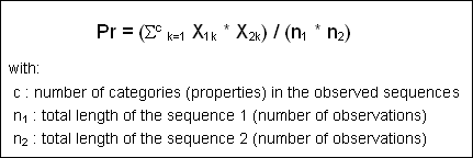
We first have to calculate Σck=1 (X1k*X2k) in the above formula:
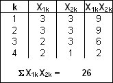
Finally Pr and Q have the following values for a sequence of 10 observations with 4 different properties:
- Pr = 26 / (10 * 10) = 26 / 100 = 0.26
- Q = 1 – 0.26 = 0.74
-
Computation of the Chi-square value for each match position p
The table below details the computation of each Chi-square value:
-
Test of significance of Chi-square value for each match position m With a degree of freedom v = 1 and a confidence level of 95%, the critical Chi-square value is 3.84.
We can then conclude that only the Chi-square value at match position -1 is significant. In other words the cross-association is significantly different from a random sequence for a negative time-shift of 1 between the two sequences. This can be observed when comparing the column “Pol. Maj. E” with the column “m-1” of “Political Majority Municipality A” in the Table 2.32. The cross-association coefficients ap for each of considered match positions can then be plotted as an associatogramme (Next figure). It shows that largest similarities between the two series occur between match positions –2 and +2.
 Associatogramme showing the successive cross-association coefficient values for match positions in the range of –7 to +7.
The two sequences are most similar with a time-shift corresponding to one year.
Associatogramme showing the successive cross-association coefficient values for match positions in the range of –7 to +7.
The two sequences are most similar with a time-shift corresponding to one year.
EXERCISE
From table expressing political majority change between municipalities A and E during the period 1900-1990 (Table) try to visually estimate:
- The two municipalities with the highest similarity at match position 0.
- Two series with a high degree of similarity but with a time shift either negative or positive.
|
|
|
|