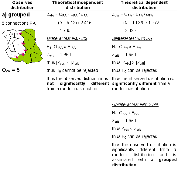
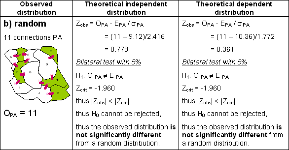
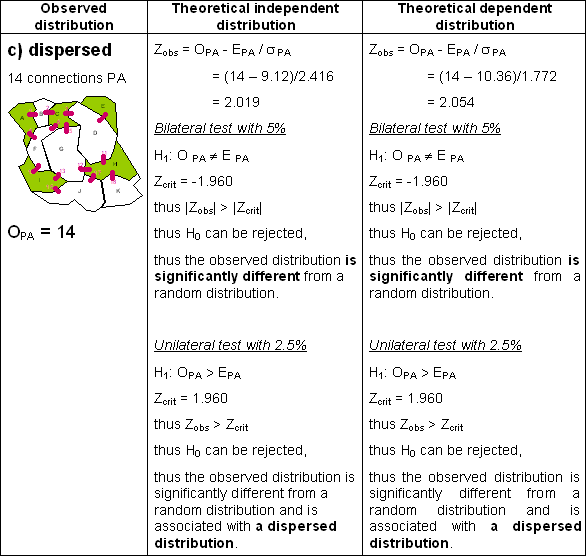
Examples of calculation for three observed spatial distributions
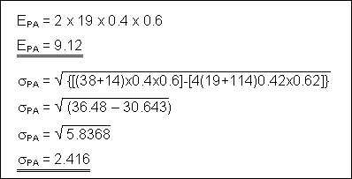
Let us take again the 3 examples of spatial distribution presented at Figure 2.4. Intuitively we can express their spatial distributions as "grouped", "random" and "dispersed". Let us test the membership of these distributions using the index of adjacency according to two situations' of independent and dependent null assumption. Being given that, in these 3 examples, we consider the same study area and that the number of zones "presence" is identical, we can calculate the two common parameters EPA and σPA for the two hypothesis, on the basis of additional information provided by the table of Figure 2.5 (C=19, ΣV=38, ΣV(V-1)=114). Whereas C = total no. of connections and V = total no. of neighbours
- For an independent null hypothesis, with a probability of occurrence "presence" p equal to 0.4 (thus q=0.6), the equations of tables 2.1 and 2.2 enable us to write:
- For a dependent null hypothesis, knowing that the number of observed events "presence" in the study area is equal to 5 per 11 zones on the whole (thus P=5 and A=6), the equations of tables 2.1 and 2.2 enable us to write:
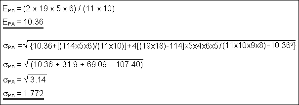
These common values being calculated, we now can operate the statistical tests relating to the two situations of independent and dependent null hypothesis considered. Let us proceed in turn for each of the three spatial distributions presented at Figure 2.4.
Tests of membership of the three types of spatial distribution of binary properties
|

