The spatial arrangement of features
According to the number and the shape of spatial features their
adjacency results in many connections, independent of their thematic property.
It is thus a question of describing this arrangement in the form of a matrix of
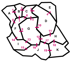
adjacencies or graphically as on figure 2.5.
Description of the spatial arrangement of areas through their adjacencies
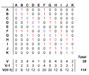
| Identification of the connections |
Matrix of adjacencies |
|
|
|
| 15 contiguous zones with 19 connections (C) |
V: number of neighbors of each area
The total number of neighbors is equal to twice the number of connections (C)
|
Figure 2.5 |
|
1.2.4a Context of the null hypothesis
The choice of the null hypothesis expresses the way in which
the properties "presence" and "absence" are assigned. From a statistical
point of view, it is a question of determining if the study area is regarded
as an independent sample (sampling with replacement, free sampling) or
dependent (sampling without replacement, non-free sampling). The identification
of one of these two situations is important because it will determine the
nature of the theoretical distribution with which the observed distribution
will be confronted.
A sample is considered independent when one knows a priori the
probability p of the property "presence" - and thus of the number of "absence",
independently of the situation observed in the area of study. For example,
in a geomorphological region including the study area, one could determine
that the probability of finding a soil of "good quality" for agriculture
is 0.4 (p=0.4, therefore q=0.6), this number being independent of the
number of zones having the property "good quality". Potentially, each zone
has same probability of 0.4 of being regarded as "good quality", whatever
the property already assigned to other zones in the study area. The estimated
random theoretical distribution will express this particular situation by
considering the parameters p and q.
A sample is considered dependent when the probability of occurrence
of the property "presence" corresponds to the proportion observed in the study
area. Returning again to the previously considered example, the situation of
dependency would correspond to the selection of the n best zones of "good aptitude"
for agriculture, among the t potential zones. The estimated random theoretical
distribution will thus take into account these parameters n and t instead of p
and q.
Generally, in practice, one gives the preference to a situation of
non-free sampling if one cannot guarantee that the estimated probability of
occurrence for the larger area is the same one as that in the study area.
Moreover, the amount of "presence" and "absence" in a study area is generally
observable and is thus given.