![]()
Examples of calculation for three observed spatial distributions
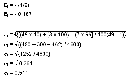
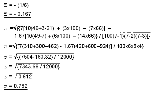
Let us return to the 3 examples of spatial distribution presented in Figure 2.6. Intuitively we can express the spatial distributions as "grouped", "random" and "dispersed" respectively. Now let’s test the membership of these distributions using the Moran’s autocorrelation coefficient according to two situations of null hypothesis, independent and dependent. Given that in these 3 examples we consider the same study area and the same set of 7 property values, we can calculate the two values EI and σI common with the three distributions for each of the two hypothesis, on the basis of additional information provided on Figure 2.7 (n = 7, C = 10, ΣV2 = 66) and in Table 2.8 below.
Calculation of indices common to the three examples |
 Table 2.8
For an independent null hypothesis, the equations of tables 2.5 and 2.6 enable us to write:
For an dependent null hypothesis, the equations of tables 2.5 and 2.6 enable us to write:
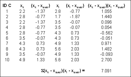
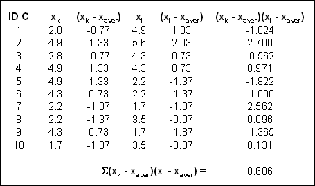
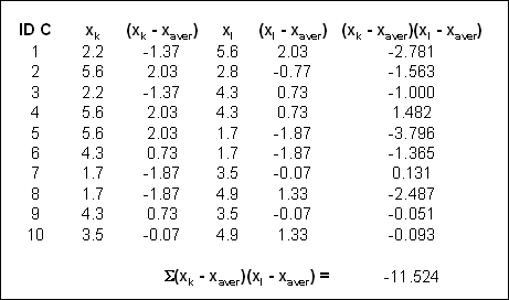
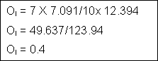
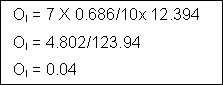
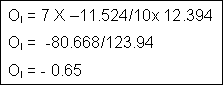
The calculation of the Moran’s coefficient for each of the three observed distributions is carried out on the basis of values produced in tables 2.8 and 2.9.
Calculation of indices specific to each of the three spatial distributions
|
|
These coefficient values being calculated, we can now carry out the statistical tests relating to the two situations of independent and dependent null hypothesis considered. Let us proceed in turn for each of the three observed spatial distributions, presented in Figure 2.6.
Tests of membership of the three types of spatial distribution of cardinal properties
|


It is observed that with a risk of error of 5%, the 3 distributions are not significantly different from a random space distribution of the values, under the hypothesis of the dependency, while only the distribution considered as grouped is significantly similar to such a spatial distribution, under the hypothesis of an independent sampling.
|
|
|
|