The Moran’s coefficient of autocorrelation (at the ordinal and cardinal level)

Many phenomena can be measured on an ordinal or cardinal level. In order to preserve informational detail of spatial feature properties, it is often interesting to turn to a spatial autocorrelation index able to take into account these ranks or these intervals of values. As one will see the formulation of the Moran’s coefficient and its application to an ordinal level of measurement is only meaningful if the rank difference has significance in its interpretation.
As for the join count statistics, the description of the spatial dependency can be expressed by the type of spatial distribution of properties within the study area: grouped, random or dispersed:

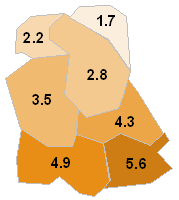
• The distribution is known as spatially grouped when properties of close value are contiguous. The spatial dependency is considered to be positively strong because the values vary in space in a "continuous" way appreciably. The spatial proximity involves a similarity of the properties (see Fig 2.6a).
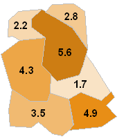
• The distribution is known as spatially random when the distribution of properties in space is unspecified. The spatial dependency is considered to be null because there is no relation between the spatial proximity and the similarity of the properties (see Fig 2.6b).
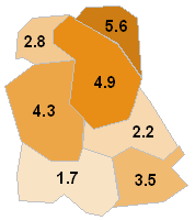
• The distribution known as is spatially random when properties of very different value are contiguous. The spatial dependency is considered to be negatively strong because the values vary in space in a "discontinuous" way appreciably. The spatial proximity involves a great difference of the properties (see Fig 2.6c).

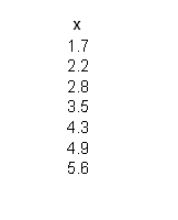
Figure 2.6 illustrates these 3 types of spatial distribution for the same study area made up of 7 zones (districts for example) on which are distributed 7 properties expressing the density of inhabitants per hectare.

Three types of spatial distribution of a set of 7 continuous properties 2.6a) grouped 2.6b) random Strong positive spatial dependency No spatial dependency 2.6c) dispersed 2.6d) 7 properties to be distributed Strong negative spatial dependency 7 values of population density per hectare Figure 2.6

The Moran’s autocorrelation coefficient, also called Moran’s I index, makes it possible to characterize the nature of this distribution according to three types (grouped, random or dispersed) and in consequence to deduce the force (strength) and the direction (positive or negative) of the spatial dependency.
Moran’s coefficient connects the differences in values between contiguous areas with reference to the total variability. Its value varies between –1 and +1. The force of the spatial autocorrelation is expressed by the value varying from 0 to 1, while the direction of the dependence is indicated by the sign, following the example of other coefficients of correlation.
Similar to the coefficient of adjacency, the definition of these differences of value between contiguous zones for a theoretical random distribution is related to two factors: spatial arrangement of zones in the study area on the one hand, and the choice of null hypothesis on the other.