![]()
The spatial arrangement of zones
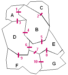
As previously shown, according to the number and the shape of the spatial features, their adjacency results in a considerable number of connections, independent of their thematic properties. The identification of connections and the neighbours for each of the 7 districts presented on Figure 2.6 is illustrated below:
Description of the spatial arrangement of the 7 districts through their adjacencies
|
1.2.8a Context of the null assumption
In the case of distribution of properties measured on a cardinal level, the two alternatives of null hypothesis presented for the join count statistic remain similar. It is thus a question of determining if the study area is regarded as an independent sample (free sampling) or dependent (non-free sampling). The identification of one of these two situations will make it possible to determine the nature of the theoretical distribution with which the observed distribution of the properties will be confronted.
On the assumption of an independent sample, one can see that the set of properties to be distributed in the study area (see figure 2.6d) results from a random sampling of a normal population; this is the hypothesis of normality.
On the assumption of a dependent sample, one considers the way of distributing the properties observed in the 7 zones, therefore one is interested in their spatial arrangement. In this case, the theoretical distribution will correspond to a random distribution; this is the hypothesis of the random distribution.
Generally, in practice, one gives the preference to a situation of dependent sampling because one usually determines the presence of the observed properties and one wishes to know the nature of their spatial distribution, i.e. to know if it is significantly different from a random distribution, therefore influenced by space.
|
|
|
|